

The Physics Behind Flow — Bernoulli, Continuity, and Pressure Drop
How Classic Laws of Fluid Dynamics Explain What You See
Last week, we launched our Tech Tuesday blog series with a deep dive into a common user question:
“Why does the pressure shown on my pump not match the pressure inside my vascular model?”
We explained how pressure drops occur as fluid passes through tubing, enters wider and more compliant vessels, and interacts with the physical structure of the simulation setup. These effects — far from being flaws — are a fundamental part of how blood behaves in real human circulation.
This week, we’re building on that foundation by exploring the classic laws of fluid dynamics that govern how blood (or simulation fluid) flows through a system. Understanding these laws isn’t just useful for simulation accuracy — it can have life-and-death consequences in clinical practice.
Some time ago, a vascular surgeon shared a case that illustrates this clearly:
“In one clinical case, surgical treatment of an abdominal aortic aneurysm was performed, including a bypass. The operation was successful and the patient was transferred to the intensive care unit in a stable condition. In the following hours, however, his condition deteriorated dramatically until he died one day after the operation due to multiple organ failure. The later autopsy revealed that the bypass had caused a reversal of the flow in the blood vessels responsible for the blood supply to the organs. Instead of transporting the blood to the organs, it was literally sucked out of them.”
This tragic outcome underscores why understanding the physics of flow — especially pressure gradients, flow direction, and vessel resistance — is critical not only for simulation but also for clinical planning and medical device design.
In this article, we’ll look at how principles like the continuity equation, Bernoulli’s principle, and Poiseuille’s law explain these phenomena, and how they apply to your simulation work.
Why Basic Physics Matters in Medical Simulation
Medical simulation often focuses on anatomy and technique — but when you’re working with pulsatile pump systems and vascular models, fluid dynamics becomes just as critical.
“Why does pressure drop when the fluid enters a wider section of the model?”
“Why does the flow rate stay the same even when the velocity changes?”
“How can narrow tubing increase pressure — and wider vessels reduce it?”
To answer these, we turn to the classic physics principles that govern real-world blood flow. This article — the second in our five-part series — explores the foundational laws behind pressure, flow rate, and vessel diameter.
The Continuity Equation: Flow Must Stay Constant
One of the core principles in fluid dynamics is the continuity equation, which tells us that for an incompressible fluid (like blood or water), the flow rate (Q) must remain constant as it moves through a closed system:
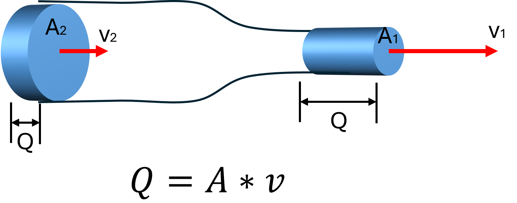
Q = flow rate
A = cross-sectional area of the vessel
v = velocity of the fluid
When fluid leaves a narrow hose (10 mm ID) and enters a larger vessel (20 mm ID), the area increases, so the velocity must decrease to maintain the same flow rate. The fluid slows down — but the volume per minute remains the same.
Bernoulli’s Principle: Energy Is Conserved, But It Shifts Forms
Bernoulli’s principle tells us that the total energy in a fluid system is constant, assuming there’s no energy loss from friction. Therefore, the flow and pressure built up by a pump is maintained in an ideal (!) fluid system. This energy has three components:
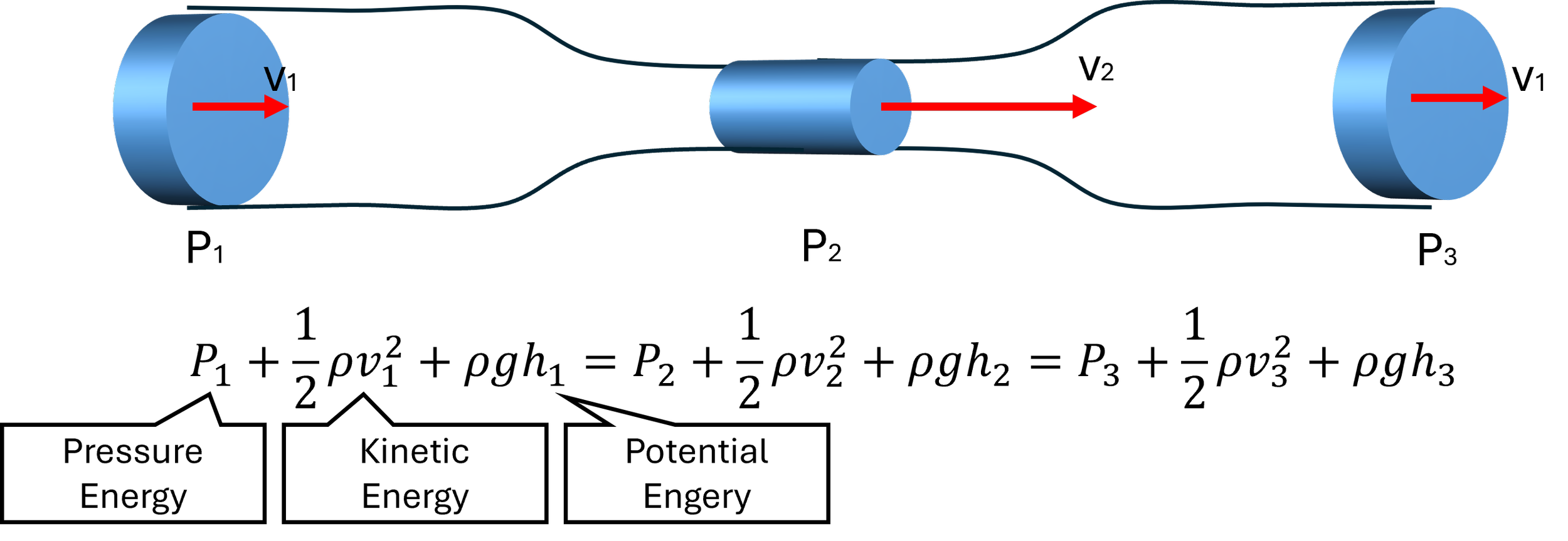
Bernoulli’s Principle
Total Energy = Sum of Pressure, Kinetic and Potential Energy
In a flat, horizontal vascular model, potential energy is negligible, so the key tradeoff is between:
Pressure energy (what you read in mmHg)
Kinetic energy (related to flow velocity)
What this means in your model:
As fluid slows down in a wider vessel (lower velocity), its pressure energy may increase in theory — but in real systems with friction and compliance, pressure typically drops due to energy loss.
Poiseuille’s Law: Resistance Rises Fast in Narrow Vessels
Poiseuille’s law describes how resistance to flow increases in narrow tubes — and how much pressure is required to overcome that resistance:

Q = volumetric flow rate (m³/s)
P = pressure (Pa)
r = radius of the tube (m)
μ = dynamic viscosity of the fluid (Pa·s)
L = length of the tube (m)
What this means in your setup:
If you halve the radius of a tube (say, from 10 mm to 5 mm), resistance increases by a factor of 16. This explains why narrower tubing or sharp connectors cause a dramatic pressure drop and why higher pump pressure is needed to maintain flow.
Laminar vs. Turbulent Flow: When Smooth Becomes Chaotic
In most simulation setups, flow remains laminar — smooth and predictable. But if velocity gets too high (e.g., with sharp transitions, tight bends, or high-pressure pulses), the flow can become turbulent, increasing resistance and pressure loss.
The Reynolds number (Re) helps determine this:
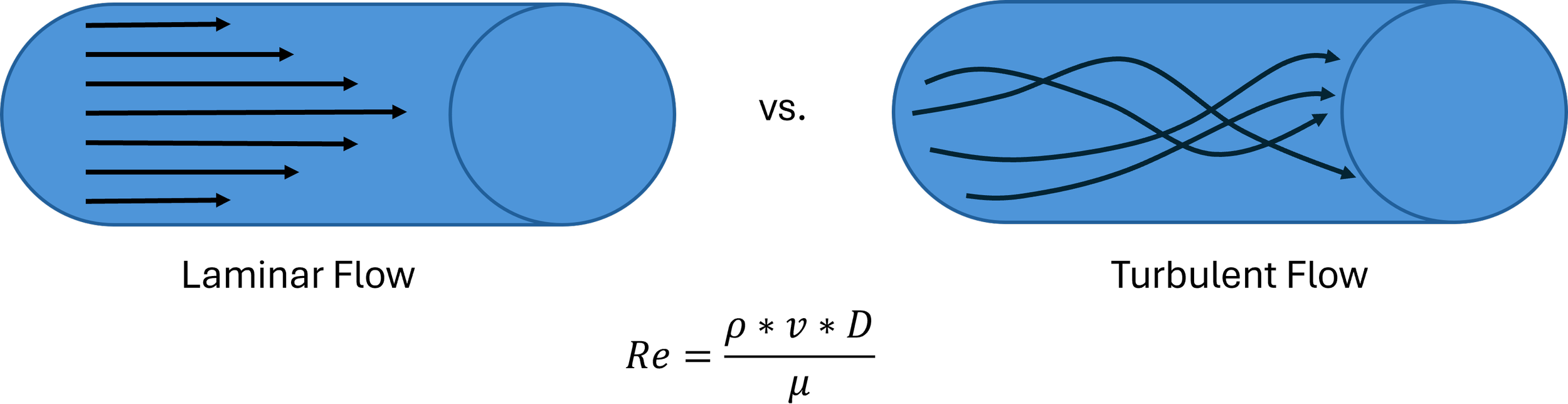
Re = Reynolds Number
ρ = fluid density
v = velocity
D = diameter
µ = viscocity of fluid
In high-Re conditions (Re > 2000), flow becomes chaotic — and simulation results may vary more due to turbulence and eddies, especially near junctions or sharp edges in your model.
Practical Example: Calculating Pressure and Velocity Changes in a Simulation Setup
Let’s walk through an example that illustrates how Poiseuille’s law, the continuity equation, and basic fluid dynamics apply to your medical simulation system.
System Setup
Pump Output: Flow rate Q = 45 ml/s = 0.000045 m³/s
Pressure at pump outlet P = 150 mmHg = 20,000 PaPTubing (inflow + outflow): Length L=0.5 m (each), Inner diameter d = 10 mm = 0.01 m
Vascular Model (e.g. Aorta): Length L = 0.6 m, Inner diameter d = 25 mm = 0.025 m
Material: Silicone (Shore D30, compliant)Fluid: Approximate viscosity μ=3.5×10^−3 Pa·s (blood simulant)

Step One: Estimate Pressure Loss in Tubing (Poiseuille’s Law)

Step Two: Estimate Flow Velocity in Each Section (Continuity Equation)
Interpretation:
The fluid slows down significantly inside the wider aorta model — from 0.57 m/s in the hose to 0.09 m/s in the model — consistent with the continuity equation.
Step Three: Estimate Remaining Pressure at Model Inlet
Total system pressure:
Pump pressure: 150 mmHg
Tubing losses (in/out): ~64 mmHg
Assume minor losses in connectors + model resistance: ~10–15 mmHg
Estimated pressure inside the model:
≈150−64−15= 70 mmHg
This means that although the pump is set to 150 mmHg, the pressure inside the aorta is closer to 70 mmHg, due to friction and expansion effects.
Step 4: Achieve 120 mmHg at the inlet of the vascular model (aorta)
Now that we know the pressure losses, we can calculate the pressure delivered by the pump to achieve 120 mmHg in the vascular model:
From our earlier calculation:
Tubing loss (inflow + outflow hoses): ~64 mmHg
Connector and model entry losses (estimated): ~10–15 mmHg
Total losses upstream of the model:
ΔPsystem ≈ 64+15 = 79 mmHg
To reach 120 mmHg inside the vascular model, you must set the pump pressure to approximately 200 mmHg.
Takeaway
Classic physics laws — the continuity equation, Bernoulli’s principle, and Poiseuille’s law — explain why flow remains constant, velocity changes with diameter, and pressure drops along the path.
When designing or using a simulation setup:
Expect slower velocity and lower pressure in wider, compliant vessels
Know that narrow tubing or long paths increase resistance and pressure loss
Use smooth, gradual transitions between connectors to prevent turbulence
These insights will help you understand and control what’s happening in your models — not just observe it.
In our next article, we’ll take a closer look at pulsatility and compliance — and how simulating the heartbeat involves more than just pushing fluid. We’ll explore how pressure waves interact with vessel walls and why timing matters just as much as flow rate.